Walmart Sales Time-Series Modeling
The following workbook was my final submission for the M5 forecasting competition hosted on Kaggle. The competition was a basic time-series forecasting challenge in which you are to predict item level sales for 9 Walmart stores across 3 states for 28 days, given 4 years of data. This was my first Kaggle competition and I finished in the 58th percentile leveraging an LGBM model and fairly simple feature engineering.
I have much experience forecasting from working in Corporate Finance, in which we forecasted business unit P&Ls. Our forecasting techniques never moved much beyond basic trending and calendarization adjustments. Since I’ve moved into the world of Data Science I’ve learned much about more advanced statistical techniques likes ARIMA modeling, but I was curious to see how Machine Learning could be applied to time-series forecasting. This competition was a great way to test out various techniques as well as learn from others about what is currently considered “State of the Art”.
After completing the competition, I’m not necessarily sold on Machine Learning for time-series forecasting over ARIMA modeling, when dealing with aggregated data. I’m not sure the accuracy improvements outweight the decrease in explainability, and increase in computational costs. Intermitent demand at the unaggregated product level was a new challenge for me, and learning to solve for this was a valuable lesson. Also, it was interesting to see several Deep Learning models perform well and I’ll keep an eye on how this develops and it’s applications in the future.
Please see below for my workbook for my final submission which used a Machine Learning approach.
Table of Contents:
- Setup
- Downcasting
- Melt
- EDA
- Feature Engineering
- Modeling and Prediction
import os
import pandas as pd
import numpy as np
import plotly_express as px
import plotly.graph_objects as go
from plotly.subplots import make_subplots
import matplotlib.pyplot as plt
import seaborn as sns
import gc
import warnings
warnings.filterwarnings('ignore')
from lightgbm import LGBMRegressor
import joblib

pd.set_option('display.max_columns', None)
pd.set_option("max_rows", None)
1. Setup
sales = pd.read_csv('/kaggle/input/m5-forecasting-accuracy/sales_train_evaluation.csv')
sales.name = 'sales'
calendar = pd.read_csv('/kaggle/input/m5-forecasting-accuracy/calendar.csv')
calendar.name = 'calendar'
prices = pd.read_csv('/kaggle/input/m5-forecasting-accuracy/sell_prices.csv')
prices.name = 'prices'
Since there is validation data available for the days 1914-1941, adding zero sales for days: d_1942 - d_1969
for d in range(1942,1970):
    col = 'd_' + str(d)
    sales[col] = 0
    sales[col] = sales[col].astype(np.int16)
2. Downcasting
Downcasting is a method that reduces memory by converting each integer field to the smallest possible integer type. In this instance, it reduces memory of df by 75%.
def downcast(df):
    cols = df.dtypes.index.tolist()
    types = df.dtypes.values.tolist()
    for i,t in enumerate(types):
        if 'int' in str(t):
            if df[cols[i]].min() > np.iinfo(np.int8).min and df[cols[i]].max() < np.iinfo(np.int8).max:
                df[cols[i]] = df[cols[i]].astype(np.int8)
            elif df[cols[i]].min() > np.iinfo(np.int16).min and df[cols[i]].max() < np.iinfo(np.int16).max:
                df[cols[i]] = df[cols[i]].astype(np.int16)
            elif df[cols[i]].min() > np.iinfo(np.int32).min and df[cols[i]].max() < np.iinfo(np.int32).max:
                df[cols[i]] = df[cols[i]].astype(np.int32)
            else:
                df[cols[i]] = df[cols[i]].astype(np.int64)
        elif 'float' in str(t):
            if df[cols[i]].min() > np.finfo(np.float16).min and df[cols[i]].max() < np.finfo(np.float16).max:
                df[cols[i]] = df[cols[i]].astype(np.float16)
            elif df[cols[i]].min() > np.finfo(np.float32).min and df[cols[i]].max() < np.finfo(np.float32).max:
                df[cols[i]] = df[cols[i]].astype(np.float32)
            else:
                df[cols[i]] = df[cols[i]].astype(np.float64)
        elif t == np.object:
            if cols[i] == 'date':
                df[cols[i]] = pd.to_datetime(df[cols[i]], format='%Y-%m-%d')
            else:
                df[cols[i]] = df[cols[i]].astype('category')
    return df

sales = downcast(sales)
prices = downcast(prices)
calendar = downcast(calendar)
3. Melt
df = pd.melt(sales, id_vars=['id', 'item_id', 'dept_id', 'cat_id', 'store_id', 'state_id'], var_name='d', value_name='sold').dropna()
##add in day of year
calendar['day_of_year'] = 0
calendar['day_of_year'] = calendar['wm_yr_wk'].astype(str).str.slice(3,5) + calendar['wday'].astype(str)
downcast(calendar)
##combine data
df = pd.merge(df, calendar, on='d', how='left')
df = pd.merge(df, prices, on=['store_id','item_id','wm_yr_wk'], how='left')
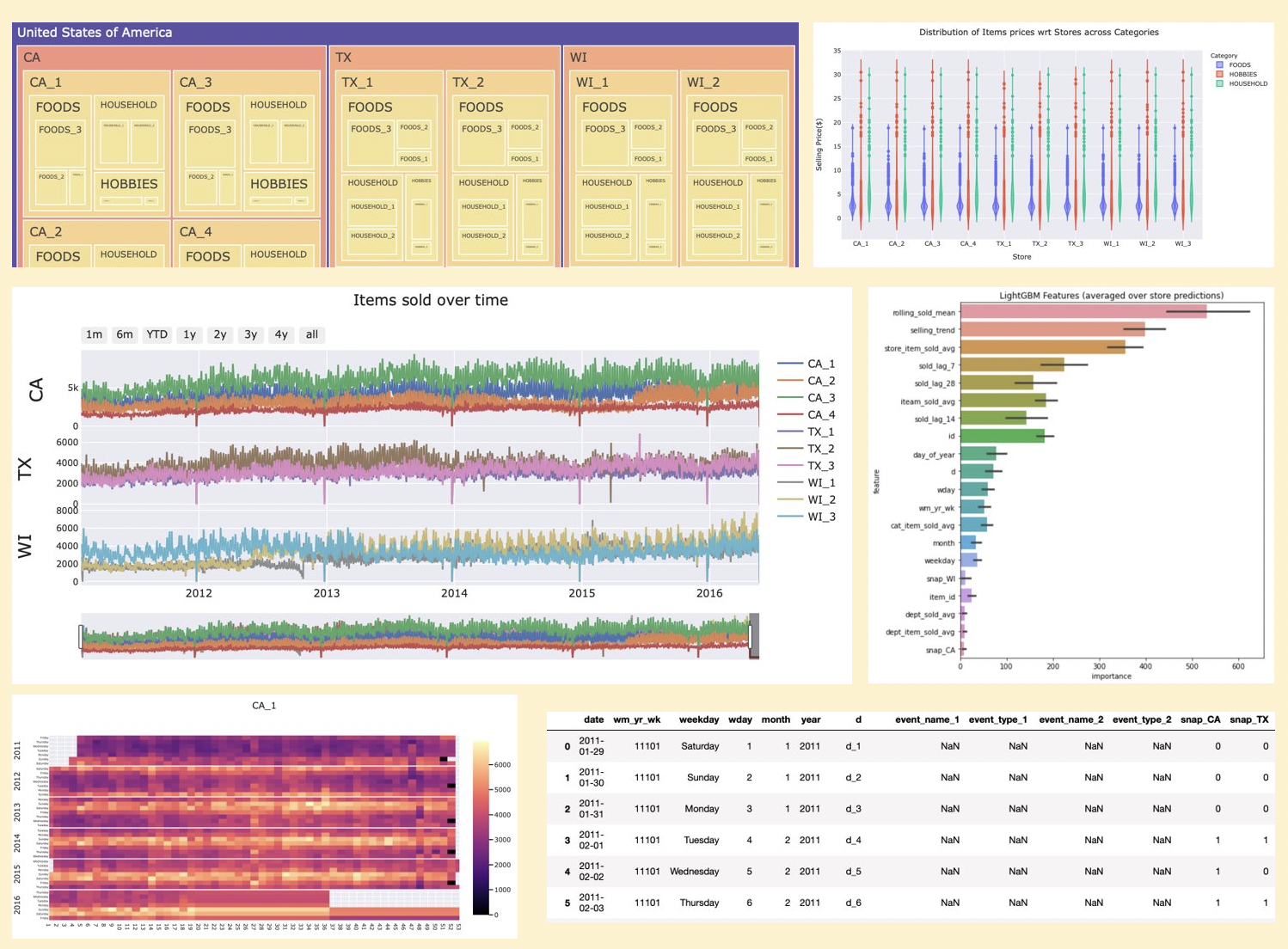
4. EDA
group = sales.groupby(['state_id','store_id','cat_id','dept_id'],as_index=False)['item_id'].count().dropna()
group['USA'] = 'United States of America'
group.rename(columns={'state_id':'State','store_id':'Store','cat_id':'Category','dept_id':'Department','item_id':'Count'},inplace=True)
fig = px.treemap(group, path=['USA', 'State', 'Store', 'Category', 'Department'], values='Count',
                  color='Count',
                  color_continuous_scale= px.colors.sequential.Sunset,
                  title='Walmart: Distribution of items')
fig.update_layout(template='seaborn')
fig.show()
Distribution of item prices by store
group_price_store = df.groupby(['state_id','store_id','item_id'],as_index=False)['sell_price'].mean().dropna()
fig = px.violin(group_price_store, x='store_id', color='state_id', y='sell_price',box=True, hover_name='item_id')
fig.update_xaxes(title_text='Store')
fig.update_yaxes(title_text='Selling Price($)')
fig.update_layout(template='seaborn',title='Distribution of Items prices wrt Stores',legend_title_text='State')
fig.show()
Distribution of item prices by store and category
group_price_cat = df.groupby(['store_id','cat_id','item_id'],as_index=False)['sell_price'].mean().dropna()
fig = px.violin(group_price_cat, x='store_id', color='cat_id', y='sell_price',box=True, hover_name='item_id')
fig.update_xaxes(title_text='Store')
fig.update_yaxes(title_text='Selling Price($)')
fig.update_layout(template='seaborn',title='Distribution of Items prices wrt Stores across Categories',
                 legend_title_text='Category')
fig.show()
Distribution of sale volume by store
group = df.groupby(['year','date','state_id','store_id'], as_index=False)['sold'].sum().dropna()
fig = px.violin(group, x='store_id', color='state_id', y='sold',box=True)
fig.update_xaxes(title_text='Store')
fig.update_yaxes(title_text='Total items sold')
fig.update_layout(template='seaborn',title='Distribution of Items sold wrt Stores',legend_title_text='State')
fig.show()
Items sold over time
fig = go.Figure()
title = 'Items sold over time'
years = group.year.unique().tolist()
buttons = []
y=3
for state in group.state_id.unique().tolist():
    group_state = group[group['state_id']==state]
    for store in group_state.store_id.unique().tolist():
        group_state_store = group_state[group_state['store_id']==store]
        fig.add_trace(go.Scatter(name=store, x=group_state_store['date'], y=group_state_store['sold'], showlegend=True,
                                   yaxis='y'+str(y) if y!=1 else 'y'))
    y-=1

fig.update_layout(
        xaxis=dict(
        #autorange=True,
        range = ['2011-01-29','2016-05-22'],
        rangeselector=dict(
            buttons=list([
                dict(count=1,
                     label="1m",
                     step="month",
                     stepmode="backward"),
                dict(count=6,
                     label="6m",
                     step="month",
                     stepmode="backward"),
                dict(count=1,
                     label="YTD",
                     step="year",
                     stepmode="todate"),
                dict(count=1,
                     label="1y",
                     step="year",
                     stepmode="backward"),
                dict(count=2,
                     label="2y",
                     step="year",
                     stepmode="backward"),
                dict(count=3,
                     label="3y",
                     step="year",
                     stepmode="backward"),
                dict(count=4,
                     label="4y",
                     step="year",
                     stepmode="backward"),
                dict(step="all")
            ])
        ),
        rangeslider=dict(
            autorange=True,
        ),
        type="date"
    ),
    yaxis=dict(
        anchor="x",
        autorange=True,
        domain=[0, 0.33],
        mirror=True,
        showline=True,
        side="left",
        tickfont={"size":10},
        tickmode="auto",
        ticks="",
        title='WI',
        titlefont={"size":20},
        type="linear",
        zeroline=False
    ),
    yaxis2=dict(
        anchor="x",
        autorange=True,
        domain=[0.33, 0.66],
        mirror=True,
        showline=True,
        side="left",
        tickfont={"size":10},
        tickmode="auto",
        ticks="",
        title = 'TX',
        titlefont={"size":20},
        type="linear",
        zeroline=False
    ),
    yaxis3=dict(
        anchor="x",
        autorange=True,
        domain=[0.66, 1],
        mirror=True,
        showline=True,
        side="left",
        tickfont={"size":10},
        tickmode="auto",
        ticks='',
        title="CA",
        titlefont={"size":20},
        type="linear",
        zeroline=False
    )
    )
fig.update_layout(template='seaborn', title=title)
fig.show()
Setup store-wise analysis
df['revenue'] = df['sold']*df['sell_price'].astype(np.float32)
def introduce_nulls(df):
    idx = pd.date_range(df.date.dt.date.min(), df.date.dt.date.max())
    df = df.set_index('date')
    df = df.reindex(idx)
    df.reset_index(inplace=True)
    df.rename(columns={'index':'date'},inplace=True)
    return df

def plot_metric(df,state,store,metric):
    store_sales = df[(df['state_id']==state)&(df['store_id']==store)&(df['date']<='2016-05-22')]
    food_sales = store_sales[store_sales['cat_id']=='FOODS']
    store_sales = store_sales.groupby(['date','snap_'+state],as_index=False)['sold','revenue'].sum()
    snap_sales = store_sales[store_sales['snap_'+state]==1]
    non_snap_sales = store_sales[store_sales['snap_'+state]==0]
    food_sales = food_sales.groupby(['date','snap_'+state],as_index=False)['sold','revenue'].sum()
    snap_foods = food_sales[food_sales['snap_'+state]==1]
    non_snap_foods = food_sales[food_sales['snap_'+state]==0]
    non_snap_sales = introduce_nulls(non_snap_sales)
    snap_sales = introduce_nulls(snap_sales)
    non_snap_foods = introduce_nulls(non_snap_foods)
    snap_foods = introduce_nulls(snap_foods)
    fig = go.Figure()
    fig.add_trace(go.Scatter(x=non_snap_sales['date'],y=non_snap_sales[metric],
                           name='Total '+metric+'(Non-SNAP)'))
    fig.add_trace(go.Scatter(x=snap_sales['date'],y=snap_sales[metric],
                           name='Total '+metric+'(SNAP)'))
    fig.add_trace(go.Scatter(x=non_snap_foods['date'],y=non_snap_foods[metric],
                           name='Food '+metric+'(Non-SNAP)'))
    fig.add_trace(go.Scatter(x=snap_foods['date'],y=snap_foods[metric],
                           name='Food '+metric+'(SNAP)'))
    fig.update_yaxes(title_text='Total items sold' if metric=='sold' else 'Total revenue($)')
    fig.update_layout(template='seaborn',title=store)
    fig.update_layout(
        xaxis=dict(
        #autorange=True,
        range = ['2011-01-29','2016-05-22'],
        rangeselector=dict(
            buttons=list([
                dict(count=1,
                     label="1m",
                     step="month",
                     stepmode="backward"),
                dict(count=6,
                     label="6m",
                     step="month",
                     stepmode="backward"),
                dict(count=1,
                     label="YTD",
                     step="year",
                     stepmode="todate"),
                dict(count=1,
                     label="1y",
                     step="year",
                     stepmode="backward"),
                dict(count=2,
                     label="2y",
                     step="year",
                     stepmode="backward"),
                dict(count=3,
                     label="3y",
                     step="year",
                     stepmode="backward"),
                dict(count=4,
                     label="4y",
                     step="year",
                     stepmode="backward"),
                dict(step="all")
            ])
        ),
        rangeslider=dict(
            autorange=True,
        ),
        type="date"
    ))
    return fig
cal_data = group.copy()
cal_data = cal_data[cal_data.date <= '22-05-2016']
cal_data['week'] = cal_data.date.dt.weekofyear
cal_data['day_name'] = cal_data.date.dt.day_name()
def calmap(cal_data, state, store, scale):
    cal_data = cal_data[(cal_data['state_id']==state)&(cal_data['store_id']==store)]
    years = cal_data.year.unique().tolist()
    fig = make_subplots(rows=len(years),cols=1,shared_xaxes=True,vertical_spacing=0.005)
    r=1
    for year in years:
        data = cal_data[cal_data['year']==year]
        data = introduce_nulls(data)
        fig.add_trace(go.Heatmap(
            z=data.sold,
            x=data.week,
            y=data.day_name,
            hovertext=data.date.dt.date,
            coloraxis = "coloraxis",name=year,
        ),r,1)
        fig.update_yaxes(title_text=year,tickfont=dict(size=5),row = r,col = 1)
        r+=1
    fig.update_xaxes(range=[1,53],tickfont=dict(size=10), nticks=53)
    fig.update_layout(coloraxis = {'colorscale':scale})
    fig.update_layout(template='seaborn', title=store)
    return fig
Flip through each store and metric (sold and revenue) to familiarize with nuances of each store.
fig = plot_metric(df,'CA','CA_1','sold')
fig.show()
Flip through each store to view sales over time by day of week
fig = calmap(cal_data, 'CA', 'CA_3', 'magma')
fig.show()
5. Feature Engineering
Label encoding:
- Remove unwanted data to create space in RAM for further processing.
- Label Encode categorical features.(I had converted already converted categorical variable to category type. So, I can simply use their codes instead of using LableEncoder)
- Remove date as its features are already present.
- Remove unecessary features.
#Store the categories along with their codes
d_id = dict(zip(df.id.cat.codes, df.id))
d_item_id = dict(zip(df.item_id.cat.codes, df.item_id))
d_dept_id = dict(zip(df.dept_id.cat.codes, df.dept_id))
d_cat_id = dict(zip(df.cat_id.cat.codes, df.cat_id))
d_store_id = dict(zip(df.store_id.cat.codes, df.store_id))
d_state_id = dict(zip(df.state_id.cat.codes, df.state_id))
#1
del group, group_price_cat, group_price_store, group_state, group_state_store, cal_data
gc.collect();

#2
df.d = df['d'].apply(lambda x: x.split('_')[1]).astype(np.int16)
cols = df.dtypes.index.tolist()
types = df.dtypes.values.tolist()
for i,type in enumerate(types):
    if type.name == 'category':
        df[cols[i]] = df[cols[i]].cat.codes

#3
df.drop('date',axis=1,inplace=True)


#4
df.drop(['revenue', 'sell_price'], axis = 1, inplace = True)
Introduce lags
#lags = [7,14,28,364,728,1092,1456]
lags = [7,14,28]
for lag in lags:
    df['sold_lag_'+str(lag)] = df.groupby(['id', 'item_id', 'dept_id', 'cat_id', 'store_id', 'state_id'],as_index=False)['sold'].shift(lag).astype(np.float16)
Mean enconding
df['iteam_sold_avg'] = df.groupby('item_id')['sold'].transform('mean').astype(np.float16)
df['state_sold_avg'] = df.groupby('state_id')['sold'].transform('mean').astype(np.float16)
df['store_sold_avg'] = df.groupby('store_id')['sold'].transform('mean').astype(np.float16)
df['cat_sold_avg'] = df.groupby('cat_id')['sold'].transform('mean').astype(np.float16)
df['dept_sold_avg'] = df.groupby('dept_id')['sold'].transform('mean').astype(np.float16)
df['cat_dept_sold_avg'] = df.groupby(['cat_id','dept_id'])['sold'].transform('mean').astype(np.float16)
df['store_item_sold_avg'] = df.groupby(['store_id','item_id'])['sold'].transform('mean').astype(np.float16)
df['cat_item_sold_avg'] = df.groupby(['cat_id','item_id'])['sold'].transform('mean').astype(np.float16)
df['dept_item_sold_avg'] = df.groupby(['dept_id','item_id'])['sold'].transform('mean').astype(np.float16)
df['state_store_sold_avg'] = df.groupby(['state_id','store_id'])['sold'].transform('mean').astype(np.float16)
df['state_store_cat_sold_avg'] = df.groupby(['state_id','store_id','cat_id'])['sold'].transform('mean').astype(np.float16)
df['store_cat_dept_sold_avg'] = df.groupby(['store_id','cat_id','dept_id'])['sold'].transform('mean').astype(np.float16)
##calc rolling window and expanding window stats

df['rolling_sold_mean'] = df.groupby(['id', 'item_id', 'dept_id', 'cat_id', 'store_id', 'state_id'])['sold'].transform(lambda x: x.rolling(window=7).mean()).astype(np.float16)
#df['expanding_sold_mean'] = df.groupby(['id', 'item_id', 'dept_id', 'cat_id', 'store_id', 'state_id'])['sold'].transform(lambda x: x.expanding(2).mean()).astype(np.float16)
Create trending: field that is a positive value if rolling average is greater than entire duration average, else negative
df['daily_avg_sold'] = df.groupby(['id', 'item_id', 'dept_id', 'cat_id', 'store_id', 'state_id','d'])['sold'].transform('mean').astype(np.float16)
df['avg_sold'] = df.groupby(['id', 'item_id', 'dept_id', 'cat_id', 'store_id', 'state_id'])['sold'].transform('mean').astype(np.float16)
df['selling_trend'] = (df['daily_avg_sold'] - df['avg_sold']).astype(np.float16)
df.drop(['daily_avg_sold','avg_sold'],axis=1,inplace=True)
6. Modeling and Prediction
##Save data in separate df in order to train separately
##cut off first 28 days because of lags

df = df[df['d']>=28]
df.to_pickle('data.pkl')
del df
gc.collect();
data = pd.read_pickle('data.pkl')
valid = data[(data['d']>=1914) & (data['d']<1942)][['id','d','sold']]
test = data[data['d']>=1942][['id','d','sold']]
valid_preds = valid['sold']
eval_preds = test['sold']
#Get the store ids
stores = sales.store_id.cat.codes.unique().tolist()
for store in stores:
    df = data[data['store_id']==store]

    #Split the data
    X_train, y_train = df[df['d']<1914].drop('sold',axis=1), df[df['d']<1914]['sold']
    X_valid, y_valid = df[(df['d']>=1914) & (df['d']<1942)].drop('sold',axis=1), df[(df['d']>=1914) & (df['d']<1942)]['sold']
    X_test = df[df['d']>=1942].drop('sold',axis=1)

    #Train and validate
    model = LGBMRegressor(
        n_estimators=1000,
        learning_rate=0.3,
        subsample=0.8,
        colsample_bytree=0.8,
        max_depth=8,
        num_leaves=50,
        min_child_weight=300
    )
    print('*****Prediction for Store: {}*****'.format(d_store_id[store]))
    model.fit(X_train, y_train, eval_set=[(X_train,y_train),(X_valid,y_valid)],
             eval_metric='rmse', verbose=20, early_stopping_rounds=20)
    valid_preds[X_valid.index] = model.predict(X_valid)
    eval_preds[X_test.index] = model.predict(X_test)
    filename = 'model'+str(d_store_id[store])+'.pkl'
    # save model
    joblib.dump(model, filename)
    del model, X_train, y_train, X_valid, y_valid
    gc.collect()
Plot feature importance
feature_importance_df = pd.DataFrame()
features = [f for f in data.columns if f != 'sold']
for filename in os.listdir('/kaggle/working/'):
    if 'model' in filename:
        # load model
        model = joblib.load(filename)
        store_importance_df = pd.DataFrame()
        store_importance_df["feature"] = features
        store_importance_df["importance"] = model.feature_importances_
        store_importance_df["store"] = filename[5:9]
        feature_importance_df = pd.concat([feature_importance_df, store_importance_df], axis=0)

def display_importances(feature_importance_df_):
    cols = feature_importance_df_[["feature", "importance"]].groupby("feature").mean().sort_values(by="importance", ascending=False)[:20].index
    best_features = feature_importance_df_.loc[feature_importance_df_.feature.isin(cols)]
    plt.figure(figsize=(8, 8))
    sns.barplot(x="importance", y="feature", data=best_features.sort_values(by="importance", ascending=False))
    plt.title('LightGBM Features (averaged over store predictions)')
    plt.tight_layout()

display_importances(feature_importance_df)
Make submission
valid['sold'] = valid_preds
validation = valid[['id','d','sold']]
validation = pd.pivot(validation, index='id', columns='d', values='sold').reset_index()
validation.columns=['id'] + ['F' + str(i + 1) for i in range(28)]
validation.id = validation.id.map(d_id).str.replace('evaluation','validation')

#Get the evaluation results
test['sold'] = eval_preds
evaluation = test[['id','d','sold']]
evaluation = pd.pivot(evaluation, index='id', columns='d', values='sold').reset_index()
evaluation.columns=['id'] + ['F' + str(i + 1) for i in range(28)]
#Remap the category id to their respective categories
evaluation.id = evaluation.id.map(d_id)

#Prepare the submission
submit = pd.concat([validation,evaluation]).reset_index(drop=True)
submit.to_csv('submission.csv',index=False)